Improving one small model: a deep look at depth-recurrence in 10-minute pretraining
We take a strong pretraining recipe and try to make it better. The recipe comes from the OpenAI Parameter Golf challenge, a small-model pretraining contest where everything except the algorithm is held fixed: the same data (FineWeb), the same hardware (8 H100s), the same 10 minutes of training, and a hard cap of 16,000,000 bytes on the final model.
Our starting point is record #1736. Before we change anything, let us understand what the model architecture looks like. Note that we will focus exclusively on the pretraining part.
The model: depth recurrence
The architecture is a depth-recurrent transformer. Most layers run once, but a contiguous band of three layers, layers 3, 4, and 5, is run as a loop: each is visited three times per forward pass (NL=2, that is two extra passes). Of the 17 layer-applications in a full forward pass, 9 of them live inside this loop band. Each pass through the band feeds the next via the plain recurrent rule
\[x_{k+1} = f(x_k)\]where each pass sees only the previous pass’s output. Laid out as a flow, the loop band repeats three times:
x → block_0 → block_1 → block_2 → [ block_3 → block_4 → block_5 ] ×3 → block_6 → ... → block_10 → output
The recurrence is meant to build better representations from the limited number of parameters we are allowed. However, it comes at a heavy time cost: the loop layers run two extra times, which is roughly 6 extra layer-equivalents on top of the baseline 11. This drops the throughput from about 8.0M tokens/s before the loop to about 5.49M tokens/s. That is a 31% drop in throughput. Is the loop worth that cost? Holding the seed and schedule fixed and turning the recurrence off, the no-loop run completes more steps but trains to a worse validation BPB. The loop earns its cost.
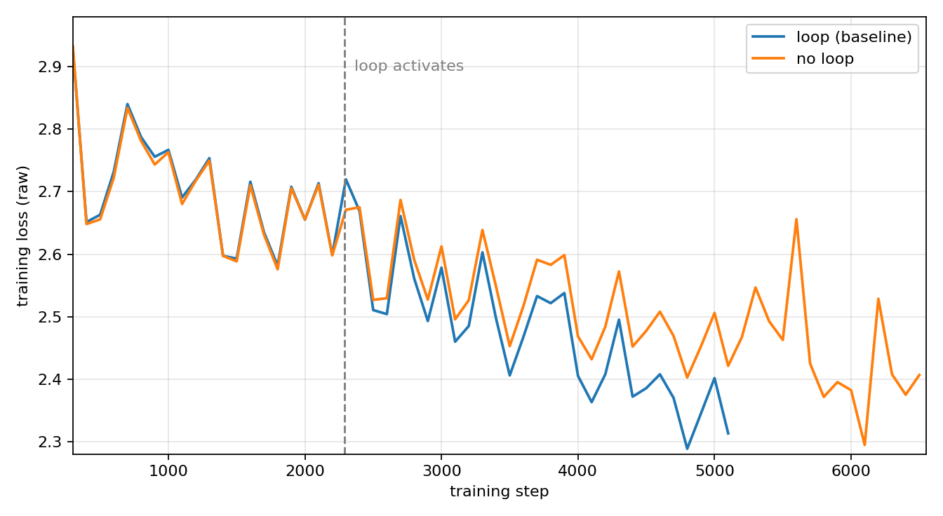
Figure 1: same seed and schedule, loop versus no loop. The no-loop run gets more steps (the loop is expensive) but the looped run trains to a lower loss and a better validation BPB.
Because it is expensive, the recipe does not run the loop from the beginning; it kicks in only at a fraction 0.35 of training. That makes it our object of study, and the three attempts below all try to improve it.
Another important piece is the learning-rate schedule, which has three phases. A short warmup ramps the rate from 0 up to its peak, which we will call LR1. It holds at LR1 only briefly. Then a long warmdown takes over for the final three quarters of training, decaying the rate linearly from LR1 back down to 0 at the end. The loop kicks in at fraction 0.35, just after the warmdown has begun, so by the time the recurrence turns on the rate has already left its LR1 peak and is on its way down.
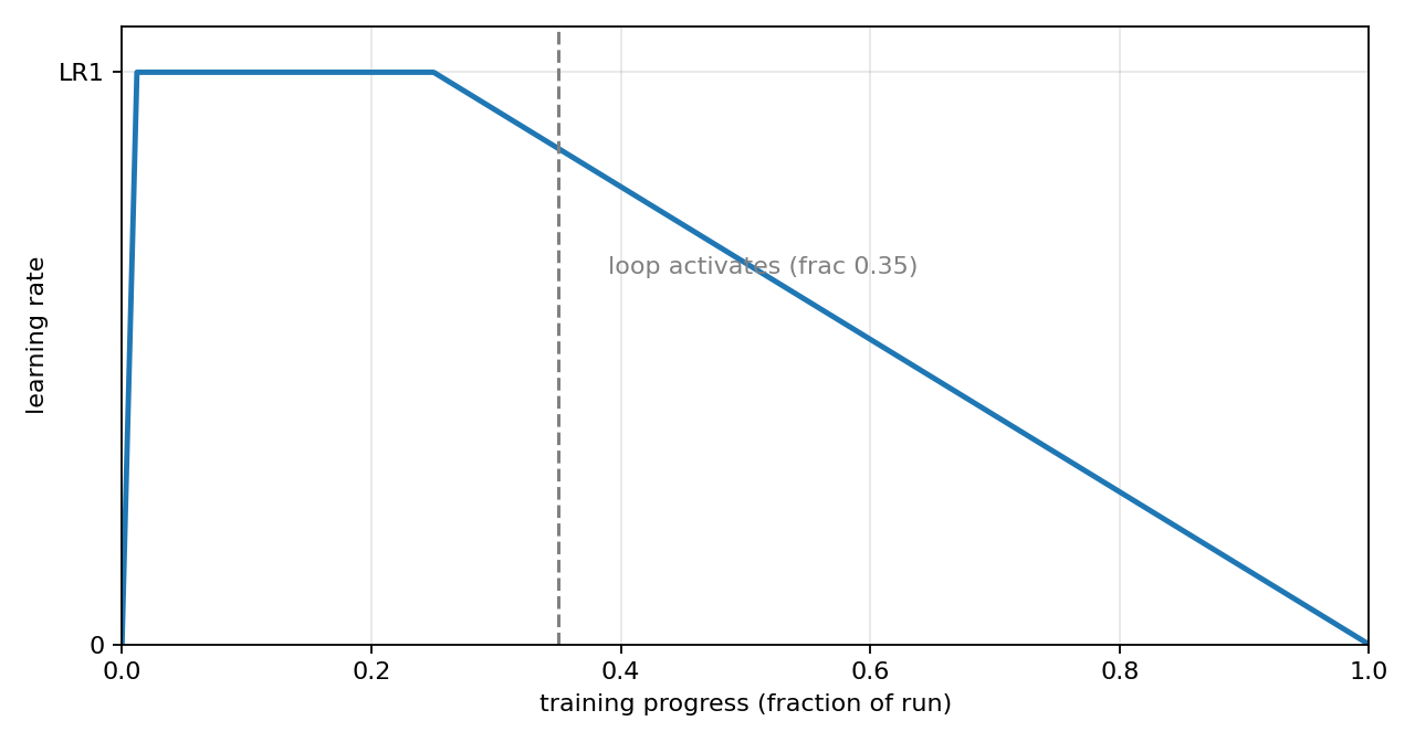
Figure 2: the learning-rate schedule. A short warmup from 0 to the peak LR1, a brief hold, then a long warmdown decaying from LR1 to 0 over the final three quarters. The dashed line marks where the loop activates, frac 0.35, just after the warmdown begins.
A quick note on the runs below: some are short screens on 4 H100s for about 20 minutes, which is the same total GPU-budget as the competition’s 8 H100s for 10 minutes, so the two are pretty comparable.
Attempt 1: when should the loop turn on?
The first attempt is to tune when the recurrence kicks in. The later it turns on, the more training steps we get to take, but at the cost of training with all three layers recurring for less of the run. A bit of quick math makes the trade-off precise. Suppose the per-step cost multiplier of the loop is \(\kappa = 1.458\) (the 46% extra work), and the loop activates at a fraction \(f\) of the budget. Let \(N_0\) be the number of steps we would complete with the loop off the whole time. The run then splits into two phases: a fraction \(f\) at the fast no-loop rate, giving \(f\,N_0\) steps, and a fraction \(1-f\) with the loop on at \(1/\kappa\) the rate, giving \((1-f)\,N_0/\kappa\) steps. So the total number of steps is approximately
\[N(f) = N_0 \left[\, f + \frac{1-f}{\kappa}\,\right],\]with the number of steps actually trained under the depth recurrence equal to \((1-f)\,N_0/\kappa\). Turning the loop on later (larger \(f\)) buys more total steps but trains with the recurrence for fewer of them.
Putting in \(N_0 = 6500\):
| kick-in \(f\) | recurrence steps \((1-f)N_0/\kappa\) | total steps \(N(f)\) | observed steps | val BPB |
|---|---|---|---|---|
| no loop | 0 | 6500 | 6500 | 1.07223 |
| 0.63 | 1650 | 5745 | 5900 | 1.06736 |
| 0.46 | 2407 | 5397 | 5700 | 1.06545 |
| 0.35 | 2898 | 5173 | 5500 | 1.06693 |
| 0.20 | 3567 | 4867 | 4800 | 1.06610 |
The predicted totals roughly track the observed counts, but the trade does not pay off. Those extra steps do not buy a better model: the no-loop run has the most steps and the worst BPB, while across the whole looped sweep the validation BPB moves by only about 0.002, with no real trend in timing. So timing the loop is not a useful lever.
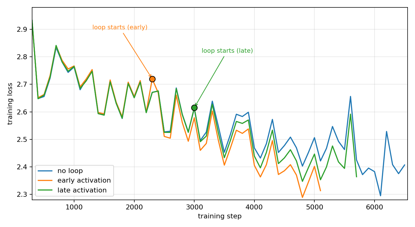
Figure 3: no loop versus early activation versus late activation, with the activation steps marked. Later activation gives more total steps, but not a better model.
Attempt 2: can the learning-rate schedule help the loop?
If we cannot improve the loop by timing it, maybe we can improve it through the schedule. We tried two moves, both shaped around the loop.
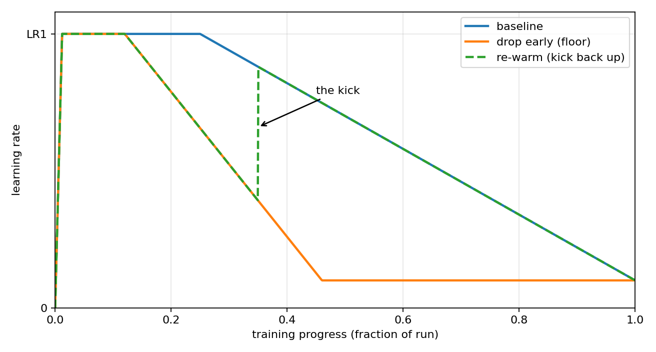
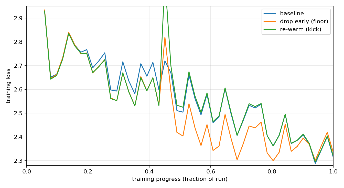
Figure 4: left, the three learning-rate schedules we tried (the baseline warmup-stable-decay; dropping the rate early and flooring it; and re-warming it back up, the kick, to rejoin the baseline). Right, their training-loss outcomes: the floored arm dips below in the middle while the re-warm arm tracks the baseline.
The first was to drop the learning rate early and floor it through the middle of training. It looks promising on training loss: the floored arm runs below the baseline through the middle of the run (Figure 4, right). But that advantage does not carry over to the metric that counts. On validation BPB, the floored arm scores 1.06800 against the baseline’s 1.06514, so the plain schedule was ahead on what mattered all along.
The second move was to kick the learning rate back up later (re-warm it). This does nothing useful, for a simple reason: once you re-warm back onto the standard schedule, the run just becomes the standard run. The re-warm arm tracks the baseline almost exactly from the re-warm point on, within about 0.0005 in training loss, and finishes at the same place.
Put together, the plain warmup-stable-decay (WSD) baseline beats every shaped schedule we tried. Here are the validation values:
| schedule | val BPB |
|---|---|
| standard WSD (baseline) | 1.06514 |
| floor then linear | 1.06598 |
| floor then WSD (re-warm) | 1.06622 |
| floor only | 1.06800 |
The best shaped schedule still loses to doing nothing by about 0.0008.
Attempt 3: change what the loop computes
This time, we change the mixing rule in the loop recurrence. Instead of the plain recurrent rule \(x_{k+1} = f(x_k)\), we give the loop a small learnable one: each pass can scale its own output and pull in carries from the other layers in the band,
\[x_{k+1} = \beta_k\, f(x_k) + \sum_j \alpha_{k,j}\, x_k^{(j)}\]initialized at \(\beta = 1\) and \(\alpha = 0\), so at the start it is exactly the plain recurrent rule. These are just a handful of scalars, trained jointly with the rest of the model.
One detail: we apply a stop-gradient (a detach) to the carried terms \(x_k^{(j)}\), so they feed the forward pass but carry no gradient backward. The main reason is speed. The loop is recurrent, so it is trained by backpropagating through every unrolled pass; if the cross-layer carries passed gradient too, each one would add another backward path through the loop and make the training slower.
When we train the models, we notice something interesting: once the loop activates, the coefficients drift off their initialization and settle into a stable pattern within a few hundred steps, and the pattern is nearly independent of initialization: runs started from \(\alpha=0\) and from \(\alpha=1\) converge to the same values.
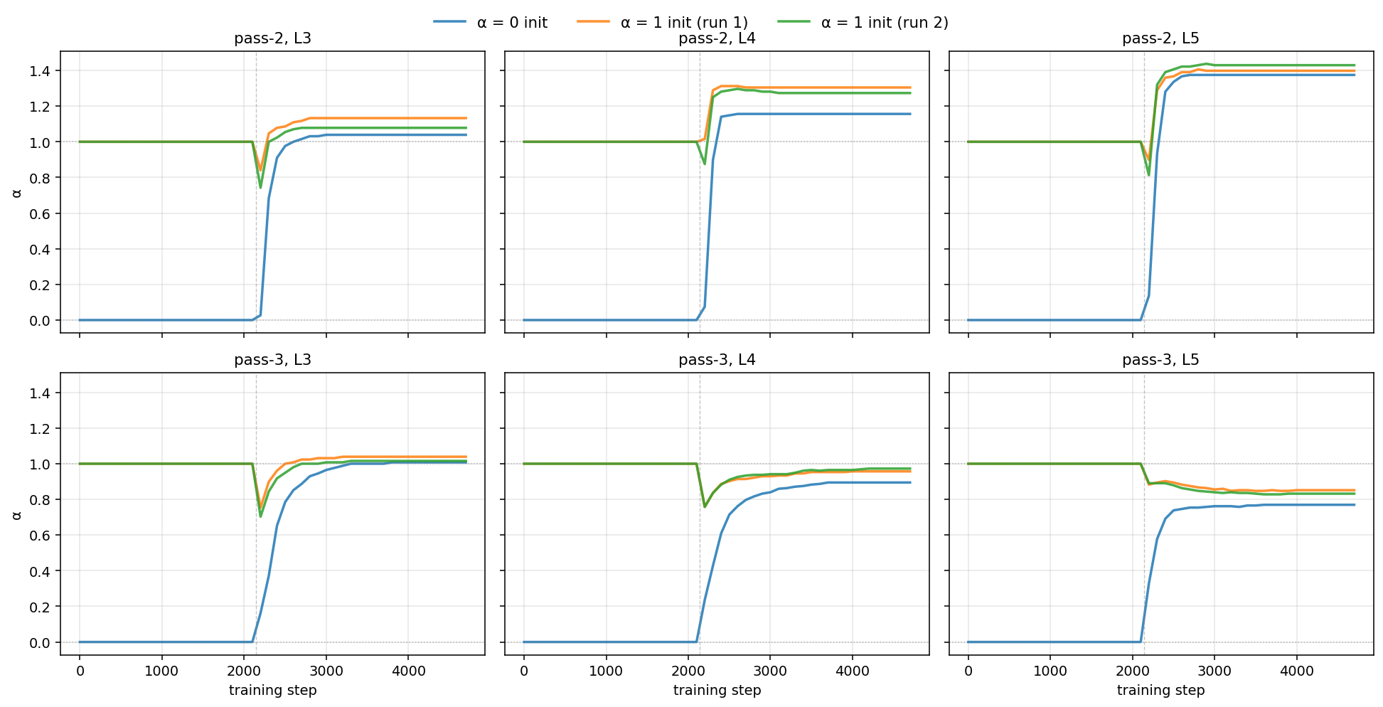
Figure 5: the alpha coefficients from runs started at different initializations all converge to the same values once the loop activates. The learned pattern is a property of the model, not of the starting point.
It is also worth looking at what the loop chose to learn. Every \(\beta\) comes out well above 1, so each pass amplifies its own block output rather than damping it; the optimizer chose to overshoot the plain recurrent rule. The cross-layer terms are structured too: layer 4 learns a self-subtract gate (its own coefficient settles near -0.35), and layer 5 acts as an aggregator, leaving itself roughly alone while absorbing a chunk of layer 4.
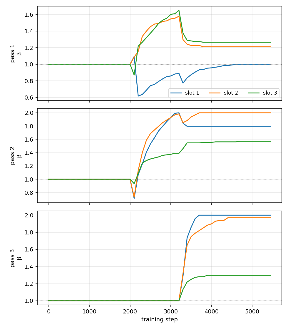
Figure 6: the per-pass beta coefficients over training, starting at 1 and drifting once the loop activates. Nearly all settle above 1, so each pass amplifies its own output.
It is therefore natural to make \(\alpha\) and \(\beta\) constants at their stabilized values. We read the converged values off the trained model and freeze them as constants in a fresh run. Freezing twelve parameters does not change the speed. What it buys is that the rest of the model trains against the stabilized values from the very start, rather than spending the early steps drifting toward them. This time, the change actually moves the competition number:
| model | mixing rule | val BPB (3-seed mean) |
|---|---|---|
| #1736 (base) | plain recurrent | 1.06549 |
| #1779 (frozen mixing) | fixed, with cross-layer carry | 1.06421 |
Later on, we also tried a slightly different variant of the same idea: an Anderson-acceleration fixed point, which extrapolates the loop from its last few iterates rather than just the previous one, frozen in the same way. It gave a similar small gain (single seed). The details are in our recurrence-band notes.
Extra: more from this competition
This was one thread of a longer competition, and the rest of it had some genuinely strange moments. There was a scoring exploit where a byte-level blend posted a sub-1.0 BPB that blew away the honest frontier while not actually being a valid probability distribution over bytes (PR #1905). And there was a validation-data leak that ran quietly across much of the leaderboard, where a default in the data-prep script put most of the validation documents into the training set (Issue #2127). We wrote those up separately; the full competition writeup is here.
Enjoy Reading This Article?
Here are some more articles you might like to read next: